Blog #32 - Types of Supernovae

Types of Supernovae

Supernovae are the most powerful known objects in the universe. Formed from old stars that collapse and explode, a supernova can emit energy on the scale of \(10^{44} \) joules, or as much energy as the Sun emits in its entire lifetime. Within a few moments of the star's collapse, it's apparent magnitude can increase by orders of 11 magnitude, often times making it the brightest object in its respective galaxy for months on end.

Supernovae are very rare occurrences and happen only once or twice per century. However in the Milky Way, only 6 have ever been recorded, the most recent being noted in 1604, before the invention of telescopes! The lack of supernovae imaging in our galaxy is due to our solar system's position in an arm of the Milky Way where most of the stars exist in the inner core. The obfuscation of light from dust and the ISM makes it nearly impossible to detect supernovae towards the center of our galaxy.

However, data from other galaxies has allowed astronomers to characterize two main types of supernovae distinguished in their light curves and process of formation. Type I supernova have a much sharper maximum peak before their light intensity gradually drops. It is believed that these types of supernova are caused by White Dwarf stars in binary systems with much larger Red Giant. The larger star gradually pulls mass from the white dwarf until it goes below a stable limit and begins to collapse on itself, causing the supernova explosion.

Type II supernova have less dramatic light curves and occur over a longer period. The progenitor star for a type II supernova is Red or Blue Supergiant. This is the more typical type of supernova and occurs when the fusion of the star's core dies out causing the gravitation equivalence to collapse and the star implodes. This explosion is typically linked to hydrogen emission lines which helps identify the type of supernova.

Blog #31 - Supernovae

Supernovae

(a) Let's estimate the energy output of a supernova. In a core-collapse supernova, the star collapses to a neutron star. A neutron star is a star/stellar remnant supported by neutron

degeneracy pressure (in contrast with white dwarfs, which are held by electron degeneracy pressure) with a diameter of ∼ 10 km and mass of ∼ 1.4 M. Using conservation of energy, we know that the energy in a supernova explosion must come from the liberation of gravitational potential energy. Estimate the energy available in a supernova explosion. Assume that the star's radius prior to collapse is 10 km.

For the first part we assume all of the kinetic energy is converted from potential energy upon explosion: \[KE = PE \rightarrow KE = \frac{3GM^2}{5R}\] Plugging in the numbers given in the problem we get \[KE = \frac{3*6.67*10^{-11}*(1.4*2*10^{30})^2}{5*10^3} = 2.1*10^{46} \space joules \]

(b) Most of the energy from part (a) is carried away by neutrinos, tiny charge less particles that rarely interact with other matter. A portion of it, however, is injected directly into the gas of the interstellar medium. When an energy E is suddenly injected to a background gas of density ρ, a strong blast wave that travels outwards is created. Using an order of magnitude estimate,show that the radius of the blast wave R scales with time t and density as R ∼ t^2/5 ρ^-1/5.
Hint: Assume that the Kinetic Energy of the blast wave is constant. Why might this be a good assumption?

Now we convert the kinetic energy of the blast into the radius that it scales to. \[KE = \frac{1}{2} m v^2 \approx mv^2\] The kinetic energy can be extrapolated by order of magnitude approximation into its components of density and radius as \[mv^2 \approx R^3 \rho (\frac{R}{t})^2 \] Which simplifies into \[KE \approx \frac{R^5 \rho}{t^2}\]Assuming the kinetic energy is constant considering that the losses in free space are negligible, we can rearrange to get [R^5 = \frac{t^2}{rho} \] or simplified to the scaling relation we expected \[R \approx \frac{t^{\frac{2}{5}}}{\rho^{\frac{1}{5}}} \]

(c) The blast wave from part (b) is known as the Sedov-Taylor blast wave, and was studied during the Second World War in the context of trying to estimate the destructive potential of the (then theoretical) atomic bomb. Use your order-of-magnitude estimate from (b) to estimate the velocity v(t) of the blast wave. Hint: Write the velocity v(t) in terms of the derivative of the radius R(t).

We know from (b) that \[R \approx \frac{t^{\frac{2}{5}}}{\rho^{\frac{1}{5}}} \] from this we can use the differential form of \(\frac{dR}{dt} = v(t) \) to solve for v(t). \[\frac{dR}{dt} = \frac{d}{dt}(t^{\frac{2}{5}}\rho^{-\frac{1}{5}}) \] Taking the derivative of the right side we get \[v(t) = \frac{2}{5} t^{-\frac{3}{5}}\rho^{-\frac{1}{5}} \]

Blog #30 - Death of a Star

Death of a Star 

1. Stellar death. We’ve now covered the main portions of a star’s life: it’s“birth” from the collapse of molecular clouds as well as the majority of it’s“life” on the Main Sequence in hydrostatic equilibrium. Now we’re going to take a look at what happens when a star like the Sun“dies” after it can no longer support itself via nuclear fusion.

(a) Life. The sun’s luminosity is L = 1033 erg/s. If fusion converts matter into energy with a 0.7%
efficiency and the Sun has 10% of its mass (the mass at the center/core) available for fusion, how long does it take to use up its fuel supply?

We start with the relationship between mass, luminosity and energy from fusion \[L \approx M^4 \approx \frac{E}{t} \] From this we can use the mass-energy equivalence to convert the energy relation to the mass of the core \[E = m*c^2 \rightarrow L \approx \frac{mc^2}{t} \] From here we can use the 0.7% conversion relation to find the time until all of the fusion energy is used. \[t = (0.007) \frac{.1 M_{\odot} c^2}{L_{\odot}} = 1.26*10^{18} seconds \approx 40 billion years\]

(b) Death. We previously derived that the time it takes for a cloud of gas to collapse under its own weight with no opposing force of pressure (i.e. the free-fall time tf f) is: \[t_{ff} = \sqrt{\frac{3 \pi}{32 G \rho}} \]

How long does it take the core of the Sun (again containing 10% of its mass) to collapse under its own weight once it runs out of fuel and there is no longer any opposing pressure?

First we solve for the density of the core \[\rho_c = \frac{M_{\odot}}{\frac{4}{3} \pi R_{\odot}^3} = \frac{3 M_{\odot}}{4 \pi R_{\odot}^3} \] Plugging this density into the equation for collapse time we get \[t_{ff} = \sqrt{\frac{3 \pi}{32 G \rho_c}} = \sqrt{\frac{\pi^2 R_{\odot}^3}{8 G M_{\odot}}} \] Solving for this value we get the time of collapse to be \[t_{ff} = 10^4 \space seconds \]This result is pretty shocking but thankfully we have fusion energy to keep our Sun alive! 

Blog #29 - Alien Megastructure

Alien Megastructure 

In 2015, a team of Yale researchers led by astronomer Tabetha Boyajian found an incredibly strange transit event occurring on the star KIC 8462852, or "Tabby's Star". Observed by the Kepler Space Telescope, KIC 8462852 showed multiple massive dips of the incoming stellar flux. Typically these types of drops signify a transiting planet but in this case the light curve peaks showed incredibly large drops of almost 20% of the incoming light. For reference, when Jupiter transits the Sun, the light curve drops only around 1% of the total flux.

Further contributing to the strangeness of the star was the dimming over time. After hearing of "Tabby's Star", researchers at Cal Tech went back to old observations of the star and found that from 2009-2013, the star displayed a drop of nearly 3% in the short time span. Of the 200 nearby comparison stars they observed, not a single one displayed such drastic results. 

These massive drops were initially contributed to a group of passive comets or planetary building blocks but as the drops showed repetitive transits, these theories were dispelled. Soon, astronomers from around the world were attempting to solve the mystery of KIC 8462852. The Search for Extraterrestrial Intelligence (SETI) is a group attempting to find life beyond our planet and currently leads research on KIC 8462852 in hopes of finding what is causing the strange light curves.

Currently the most exciting theory surrounding Tabby's Star is that of the alien megastructure. Though mostly speculation, SETI and other alien optimists believe that a large intelligently made structure surrounds the star, rotating to collect the energy from the stellar structure. They believe that the "megastructure" blocks the outgoing light of the star for large portions of the orbit, causing the severe drops in the incoming light. 

Unfortunately further research into the megastructure has come up empty. Both radio and infrared telescopes were pointed at the structure in hopes of receiving outgoing signals or "waste heat" if the structure was in fact absorbing heat from the central star. Neither was found and astronomers more or less gave up on the idea that there was a circumstellar structure around Tabby's Star. 

Still the hunt continues to try and identify what was happening in 2015 at Yale. Most astronomers now agree that the curves were probably distorted by some phenomena of the interstellar medium, though no evidence has proven this hypothesis either. 

Blog #28 - Habitable Zone pt. 2

Habitable Zone pt.2

2. In this problem we’ll figure out how the habitable zone distance, Ahz, depends on stellar mass. Recall the average mass-luminosity relation we derived earlier, as well as the mass-radius relation for stars on the main sequence. If you don’t recall, this is a good time to practice something that will very likely show up on the final!

(a) Express aHZ in terms of stellar properties as a scaling relationship, using squiggles instead of equal signs and ditching constants.

Simplifying the answer from part one, we get the relation \[T_p \approx C*L_s^{\frac{1}{4}}*a_{hz}^{\frac{1}{2}} \]Rearranging for a we get \[a_{hz}^{\frac{1}{2}} \approx C*L_s^{\frac{1}{4}}*T_p^{-1}\]Which gives us \[a_hz \approx C*L_s^{\frac{1}{2}}*T_p^{-2} \]

(b) Replace the stellar parameters with their dependence on stellar mass, such that aHZ ∼ Mα. Find α.

From an earlier worksheet we know the relation that \[L_s \approx M_s^4 \] This relation can help turn the semi major axis into a number based solely on the physical makeup of the star and planet. From part (a) we have \[a_hz \approx \frac{L^{\frac{1}{2}}}{T_{hz}^{2}} \approx \frac{M_s^{2}}{T_{hz}^{2}}\]

(c) If the Sun were half as massive and the Earth had the same equilibrium temperature, how many days would our year contain?

Converting this to a relationship for the orbital period, we have \[P^2 \approx \frac{a^3}{M_s}\] Substituting in our term for \(a_{hz}\) we get \[P^2 \approx \frac{(\frac{M_s^2}{T_{hz}^2})^3}{M_s} \]Using the information that \(T_{hz}\) is the same and \(M = .5 M_s \) we get \[P^2 \approx \frac{(\frac{\frac{1}{2}M_s^2}{T_{hz}^2})^3}{\frac{1}{2}M_s} \approx \frac{\frac{1}{64}M_s}{\frac{1}{2} M_s} \rightarrow P \approx \sqrt{\frac{1}{32}}*P_E \]Giving us a final answer of \[P \approx \sqrt{\frac{1}{32}}*365 \space days = 64.52 \space days \]

Blog #27 - Habitable Zone pt.1

Habitable Zone Pt. 1

The Earth resides in a “Goldilocks Zone” or habitable zone (HZ) around the Sun. At our semi major axis we receive just enough Sunlight to prevent the planet from freezing over and not too much to boil off our oceans. Not too cold, not too hot. Just right. In this problem we’ll calculate how the temperature of a planet, Tp, depends on the properties of the central star and the orbital properties of the planet.

(a) Draw the Sun on the left, and a planet on the right, separated by a distance a. The planet has a radius Rp and temperature Tp. The star has a radius R and a luminosity L and a temperature Teff.

We begin by putting together a picture of the setup, seen below: 

(b) Due to energy conservation, the amount of energy received per unit time by the planet is equal to the energy emitted isotropically under the assumption that it is a blackbody. How much energy per time does the planet receive from the star?How much energy per time does the Earth radiate as a blackbody?

We start by finding the amount of energy incident on the planet. This number comes from the amount of flux that hits the planet's surface. \[F_s = \frac{L_s}{4 \pi a^2}\] \[E_{in} = F_s * \pi R_p^2 = \frac{L_s R_p^2}{4 a^2} \]We then solve for energy coming out of the planet as simply the luminosity out of the surface of the Earth. \[E_{out} = L_p = \sigma T_p^4 (4 \pi R_p^2)\]

(c) Set these two quantities equal to each other and solve for Tp.

Setting the two energies equal to each other gives us: \[E_{in} = E_{out} \rightarrow \sigma T_p^4 (4 \pi R_p^2) = \frac{L_s R_p^2}{4 a^2}\] Rearranging for \(T_p\) we get \[T_p = (\frac{L_s}{16 \pi a^2 \sigma})^{\frac{1}{4}} \]

(d) How does the temperature change if the planet were much larger or much smaller?

Notice that this equation does not depend on the size of the planet so the distance is inherently based on the distance from and luminosity of the star. 

(e) Not all of the energy incident on the planet will be absorbed. Some fraction, A,will be reflected
back out into space. How does this affect the amount of energy received per unit time, and thus how does this affect Tp?

By adding a term for reflectance the \(E_{in}\) becomes \[E_{in} = \frac{L_s R_p^2}{4 a^2}*(1-A)\] Meaning that our \(E_{in}\) will not reach the full flux of the star incident to the planet. This means that the energy out of the planet will also have to decrease meaning the overall temperature of the planet will decrease as well.

Blog #26 - Angular Momentum

Angular Momentum




1. Angular momentum. In this problem we will obtain some intuition on why a disk must form during star formation if angular momentum is to be preserved.

(a) Cloud angular momentum. Consider a typical interstellar cloud core that forms a single star. You can assume it has a mass of 1 M and a diameter of 0.1 pc. A typical cloud rotational velocity is 1 m/s at the cloud edge. Calculate the angular momentum of the cloud assuming constant density. If the core collapses to form a sunlike star, what would the velocity at the surface of the star be if angular momentum is conserved? How does this compare with the break-up velocity of the Sun which is ∼300 km/s?

We begin by finding the equation for the angular momentum, L. We know we can relate the moment of inertia for a sphere and angular velocity to their linear equivalents to turn rotational movement into instantaneous linear movement. \[L = I \omega = M R v \] Using the information in the problem we can equate the rotational speed of the gas cloud and the speed of the rotating star to find the speed at the surface of the star. \[M_{\star} R_{\star} v_{\star} = M_{cloud} R_{cloud} v_{cloud} \] We know the cloud and the sun-like collapsed star have roughly the same mass so our equation for the speed of the star surface becomes \[v_{\star} = \frac{R_{cloud} v_{cloud}}{R_{\star}} \] Plugging in the given values we get \[v_{\star} = \frac{.05 pc*1 \frac{m}{s}}{2.3 * 10^{-8} pc} = 2170 \frac{km}{s} \] This value is much higher than the given \(300 \frac{km}{s}\) for the Sun. 

(b) Disk angular momentum. Assume that all the angular momentum is instead transferred to a disk of size 10 AU and negligible height. How massive must the disk be? You can assume constant density. (Hint: You can assume that the disk rotates with a Keplerian velocity given by v = GM/r where M is the mass and r is the radius.)

We again begin by solving for the rotational inertia by equating the moment of inertia and velocity of a sphere (star) to the inertia of the disk. \[L_s = \frac{2}{5} M_s R_s v_s  = \frac{1}{2} M_d R_d v_d = L_d \] We also know that the speed of the disk can be described by Keplerian velocity so we substitute \[L_d = \frac{1}{2} M_d R_d * (\sqrt{\frac{G M_s}{R_d}}) \] Notice the mass of the velocity term is dictated by the central star as it is assumed to be much more massive than the surrounding disk material. Simplifying and solving we get \[M_d = \frac{4 (M_s)^{\frac{1}{2}} R_s v_s}{5 (R_d)^{\frac{1}{2}} G^{\frac{1}{2}}} \]Solving for our constants, we get \[M_d = 1.71*10^{29} \space kg \]

(c) Solar System. The Sun has a surface rotational velocity of ∼2 km/s at the equator. How do the angular momenta of the Sun and Jupiter compare?

Comparing the angular momentums \[\frac{L_s}{L_j} = \frac{M_s R_s v_s}{M_j R_j v_j}\] which gives us a ratio of around 18 times the angular momentum for the Sun given the sun moves at around 2 km/s and Jupiter moves around 12 km/s.

Blog #25 - Sphere of Influence vs. Hill Sphere

Sphere of Influence vs. Hill Sphere

Beyond the Hill Sphere, which dictates the maximum orbital distance a satellite body can be around its host planet, planets have another astrodynamic factor called the Sphere of Influence (SOI).

The Sphere of Influence has a similar definition to the Hill Sphere but dictates how far an orbiting body from a planet can be for the planetary body to still have the dominant gravitational effect on it, compared to the much larger, further stellar body.

The Sphere of Influence has a derivation based on the 3-body problem between a star, planet, and orbiting body. The 3-body problem dictates how three orbiting bodies will move with one another based on patched conics, or the interplay of eccentricity and orbit shape.

The SOI has a complicated derivation but ends up with a very similar form to the Hill Sphere at \[R_{SOI} = a * (\frac{m}{M})^{\frac{2}{5}}\] Where a is the planet’s semi-major orbital axis, m is the mass of the planet, and M is the mass of the star. This equation is very similar to the Hill Sphere which holds as \[R_{Hill } = a * (\frac{m}{3M})^{\frac{1}{3}} \] The only difference as we see is the exponential factor and a constant in the denominator.

While the Hill Sphere tells how far an orbiting satellite or moon can sit around a central planet, the SOI dictates which body (the planet or the star) should dictate the orbiting body’s motion. Within the SOI of a planet, the patched conics orbital mechanics approach will be based on the mass and distance to the planet, without considering the massive star, as it is not the dictating gravitational player in the system.

Blog #24 - Hill Spheres

Hill Spheres

One outcome of planet formation is systems of satellites around planets. Now you may ask yourself, why do some planets have moons 10s of millions of kilometers away, while the Earth’s moon is only 400,000 km away. To answer this question we need to think about how big of a region around a planet is dominated by the gravity of a planet, i.e. the region where the gravitational pull of the planet is more important than the gravitational pull of the central star (or another planet). 

(A) Gravitational forces. Put a test mass somewhere between a star of mass Ms and a planet of mass mp at a distance rp from the star. Make a drawing marking clearly these characteristics as well as the distance r between the test particle and the planet. Write separate expressions for the gravitational force on the particle from the star and on the particle from the planet. At what distance r from the planet are the two forces balanced? This distance approximates the radius of the Hill sphere, which in the case of planet formation is the sphere of disk material which a planet can accrete from. 

We begin by drawing out the situation described in the problem 

From the drawing we need to balance gravitational forces between the star and the planet both acting on the orbiting particle or satellite. It's important to note that the balance has to exist on all sides of the particle's orbit around the planet. \[\frac{G M_s}{(R_p - R)^2} - \frac{G M_s}{(R_p + R)^2} = \frac{G M_p}{R^2} \] Cancelling G and simplifying both sides we get \[\frac{4 M_s R_p R}{R_p^4 - 2 R_p^2 R^2 + R^4} = \frac{M_p}{R^2} \] Because R is much smaller than \(R_p\) we can simplify the left side of the equation to \[\frac{4 M_s R}{R^3} = \frac{M_p}{R^2} \] Then by rearranging to solve for R we get \[R = R_p (\frac{M_p}{4 M_s})^{\frac{1}{3}}\]However the true equation for Hill Sphere differs by a constant factor due to orbital rotation speeds and comes out to \[R = R_p (\frac{M_p}{3 M_s})^{\frac{1}{3}}\]

Plugging constants from the table into the equation above, we get \[R_{Earth} = 1.49*10^6 \space km \quad R_{Jupiter} = 5*10^7 \space km \quad R_{Neptune} = 1.15*10^8 \space km \]Comparing these values to the values for the furthest moon around each planet it becomes clear that each moon is well within the planet's Hill Sphere. 

Blog #23 - History of ISM

History of ISM

The interstellar medium, or ISM, is one of the more complicated phenomena in the universe. Interestingly, the first mention of ISM was back in 1626 quoted by English explorer Francis Bacon as he stated "The Interstellar Skie.. hath .. so much Affinity with the Starre, that there is a Rotation of that, as well as of the Starre." Later, English philosopher Robert Boyle (of Boyle's law) claimed "The inter-stellar part of heaven, which several of the modern Epicureans would have to be empty." 

These early reports showed that even with primitive technology, early philosophers and astronomers were able to deduce that the space between the stars and planets in the night sky was not mere emptiness. However, for centuries, scientists believed there was an luminiferous ether that moved light throughout the universe but did not have any quantitative data as to how electromagnetism or quantum physics operated. 

In 1904, after the advancement of absorption spectroscopy, Johannes Hartmann, a German physicist, made the first observation of cold diffuse matter. This matter, later to be described as the Interstellar Medium was found as Hartmann observed the light curves of Delta Orionis. He saw that the "k" line of calcium appeared far too faint given the observing conditions and surrounding spectra. He concluded that much of the light must have been absorbed before entering Earth's atmosphere. 

Within the next decade, research into the ISM exploded and various researchers helped categorize ISM as clouds with doppler shifts. Then the discovery of cosmic rays confirmed that with the incredibly number of stars in the Universe there could statistically not exist an absolute vacuum and some medium would need to exist to absorb and transfer the massive amounts of cosmic rays, ionized hydrogen, and other basic elements that exist throughout the universe.

Today NASA has developed much of the theory behind the ISM but still lacks the knowledge to fully develop the development, growth, and existence of ISM. We now know that ISM interacts with polycyclic aromatic hydrocarbons (PAHs) to create the earliest forms of organic matter that may help shape how the big bang developed into life as we know if today. If these connections are confirmed, ISM will truly be responsible for all life as we know it.

Blog #22 - Stromgren Sphere

Stromgren Sphere

A) Set up an equation of the size of a sphere that is ionized around a star assuming uniform photon flux in all directions, and uniform density in terms of the total ionization rate \( \eta\), the density \(n\) and the recombination cross section \(\alpha\). Assume that all recombinations result in photons that cannot ionize anything further. At steady state the total photoionization rate \(\eta\) is balance by the total recombination rate.

Given the steady state assumption, we can begin by solving for \(\eta\) the recombination rate, by simple unit conversion. We know from the previous post that the recombination rate, r, is \[r = n_e * n_p * \alpha \space [\frac{1}{s \cdot cm^3}] \]We know that the number of electrons and protons must be equal if the sphere is uniformly atomic hydrogen. \[n_e = n_p \rightarrow r = n^2 \alpha\]We want \(\eta\) in terms of \(\frac{1}{s}\) meaning we need to multiply by the volume of the total sphere, given that the ionization (and recombination) occurs equally in all directions. \[\eta = n^2 \alpha V = \frac{4}{3} \pi r_{ss}^3 n^2 \alpha \]Rearranging to solve for \(r_{ss}\), the radius of the Stromgren Sphere, we find \[r_{ss} = (\frac{3 \eta}{4 n^2 \alpha \pi})^{\frac{1}{3}}\]

B) Calculate the total number of ionizing photons emitted per second by the kind of star identified in the previous problem assuming its entire luminosity is due to photons with exactly the energy required for ionizing hydrogen atoms.

This problem asks us to solve \(\eta\) which is a rate in units \(\frac{photons}{second} \). To do this we relate the luminosity of the star from the previous problem to \(\eta\). We know that the luminosity is the amount of energy emitted by the surface of a star every second. \[L = 4 \pi r^2 \sigma T^4 \space [\frac{erg}{s}] \] From the given table we find that for an O type star (temperature >30,000K). \[r_{star} \approx 10*R_{\odot} = 6.96*10^{11} cm\]With this information we solve the luminosity \[L = 4 \pi r^2 \sigma T^4 \space [\frac{erg}{s}] = 3.92*10^{38} \frac{erg}{s}\]To convert this into the rate we need, we simply divide by the energy of a single ionizing photon, \(2.17*10^{-11} erg\). \[\eta = \frac{L}{2.17*10^{-11} erg} = 1.8*10^{49} \frac{photons}{second} \]

C) With information from (A) and (B), what is the size of a Stromgren Sphere around this kind of star assuming an initial hydrogen atom density of \(1 cm^{-3}\). The recombination rate \(\alpha = 3*10^{-9} cm^{-3} s^{-1}\). How does your answer compare to the HII region of Orion, which is ionized by a few massive stars and is 8pc across?

Plugging in the \(\eta\) from (B) into the equation for \(r_{ss}\) from (A) we can solve for the radius of the Stromgren Sphere. \[r_{ss} = (\frac{3 \eta}{4 n^2 \alpha \pi})^{\frac{1}{3}} = \frac{3 * 1.8 * 10^{49}}{4* 1^2 * 3*10^{-9} * \pi} = 1.57 * 10^{57} cm \approx 5pc \]Our answer is expectedly smaller than the Orion system which has a few massive stars ionizing the HII region.

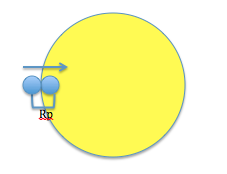
D) Make a drawing of the Stromgren sphere surrounded by the neutral HI region. What is the size of the transition region at the edge of the Stromgren Sphere where atomic hydrogen and protons co-exist? How does the size of the transition region compare with the radius of the sphere? Does it make sense to think about the HI and HII regions as distinct?

From the drawing and the information given in the problem it becomes evident that to find the size of the transition area we must calculate the mean-free-path to find the width of the area in which hydrogen protons will be ionized by photons. If this path length is very large, the two areas could be considered distinct, whereas if it is small, much of the HI region will continue to be ionized by the photons that cross the transition region. We calculate mean-free-path \[l = \frac{1}{n * \alpha} \]Where n is the particle density and \(\alpha \) is the ionization cross-section as defined in the earlier section. \[l = \frac{1}{1*3*10^{-9}} \approx 3*10^8 cm\]This transition zone is significantly smaller than the the Stromgren radius of 5pc, thus we consider the two regions as non-distinct and expect interaction along the edge of the radius.

Blog #21 - Hydrogen Ionization

Hydrogen Ionization 

A) The most abundant species in the ISM outside of molecular clouds is atomic hydrogen. We need to determine how hydrogen is ionized in order to determine properties of the ISM. Make a drawing of the electronic energy levels of atomic hydrogen. Mark out the energy needed to excite an atom in its ground state to a free proton and electron. Illustrate what happens in the case of photoionization.

http://dev.physicslab.org/Document.aspx?doctype=3&filename=AtomicNuclear_BohrModelDerivation.xml

When the hydrogen atom receives enough energy from incoming light to jump up 13.6 eV in energy, it escapes it's atomic structure and ionizes into a proton and an electron. 

B) Remember that stars are blackbodies. Which kind of stars emit a majority of their protons with energies high enough to photoionize (excited the electron to freedom) ground state hydrogen. Give your answer in both stellar temperature, and letter classification. 

To solve for the temperature needed to create a 13.6 eV increase in energy we can simply use Planck's law and Wein's displacement law. First we know \[E = \frac{h c}{\lambda}\] which gives us \[13.6 eV = \frac{4.135*10^{-15} * 3*10^8}{\lambda} \rightarrow \lambda = 91.2 nm = 912 angstrom \]With this wavelength we can use the Wein displacement law to solve for temperature. \[\lambda T = 3 * 10^{-3} m \cdot K\] From here we can solve for temperature of our blackbody. \[T = \frac{3*10^{-3} m \cdot k}{91.2*10^{-9} m} = 32894 K \]This very high surface temperature gives the star an O Type classification on the Morgan-Keenan scale. 

C) The ionization cross section is \(10^{-17} cm^2 \). Calculate the photon flux assuming the you are sitting right next to the star from (B) and that the star is emitting all of its energy in the form of photons with the exact energy required to ionize atomic hydrogen. How does this time scale compare to the excited time scale of a hydrogen atom, \(10^{-9} s \)? Is it reasonable to assume that all hydrogen is at the ground state? 

We begin with the Stefan-Boltzmann law to relate the stellar flux to the temperature of the star. \[\sigma T^4 = F \rightarrow (5.67*10^{-5} \frac{erg}{s \cdot cm^2 \cdot K^4} * (32894 K)^4 = 6.64*10^{13} \frac{erg}{s \cdot cm^2} \] Using simple unit conversion we can find our timescale from this result by multiplying by an area (to cancel the cm^2) and dividing by an energy (to cancel the ergs).\[6.64*10^{13} \frac{erg}{s \cdot cm^2} * 10^{-17} cm^2 * \frac{1}{13.6eV = 2.18*10^{-11} erg} = 3.05*10^7 \frac{photons}{second} \]Converting this to a timescale through inversion we get \[3.05*10^7 \frac{photons}{second} = 3.28*10^{-8} \frac{seconds}{photon} \] This time scale is larger than the \(10^{-9}\) excited state lifetime meaning that the photon will almost always fall back to its ground state before the next photon has the chance to ionize the atom to its next energy level. 

D) Draw a recombination event. Set up an equation for the recombination rate, r (which has units of cm^3 s^-1), in terms of the number densities of photons, electrons (np and ne) and the rate coefficient \(\alpha\), which describes the efficiency at which a recombination occurs when an electron and proton collide. 

http://hendrix2.uoregon.edu/~imamura/123/lecture-6/recombination.jpg

To solve for the recombination rate, we simply need to match units. We know \[n_p = \frac{protons}{cm^3} \quad n_e = \frac{electrons}{cm^3} \quad \alpha = \frac{cm^3}{s}\] Thus if we want a rate in terms of \(\frac{1}{cm^3 \cdot s} \) we simply need to multiply the three terms. \[r = n_p * n_e * \alpha \]

Blog #20 - What is TRAPPIST?

What is TRAPPIST? 

A lot of excitement was generated on February 22, 2017 when NASA released a press statement announcing the founding of 7 exoplanets orbiting a star 12 parsecs from Earth. Using transit photometry, as discussed in earlier blog posts, the Transiting Planets and Planetesimals Small Telescope (TRAPPIST) was able to record the presence of 7 exoplanets around a single star, 5 of which appear to be in or around the habitable zone while 3 have roughly Earth-sized radii.

TRAPPIST is actually a system of two 60-cm reflective, optical telescopes. The first, TRAPPIST-South is located in the Chilean mountains at La Silla Observatory while TRAPPIST-North is located in the Atlas Mountains of Morocco. Despite their locations, both telescopes are controlled out of Liege, Belgium and operate under fully autonomous, robotic systems. The team of telescopes creates photometry data by observing when planets transit across their host stars, causing an observed drop in incoming flux. The plot below shows the process for determining the transit of a planet which helps determine its period, radius, and location around a star.

When it came to the 7 planets orbiting TRAPPIST-1, the photometry data was truling startling as the 7 planets all created well defined transit drops. Below is the aligned data for all 7 planets as well as the brightness plots and a schematic of the orbits for the star system. 

The bottom left image is the aligned 7 photometry plots with clear ingress and egress dips and corresponding transit depths. These images in conjunction with the TRAPPIST telescopes were imaged by the Spitzer Space Telescope. 

Blog #19 - Transiting Exoplanet pt. 2

Transiting Exoplanet pt. 2

2. Now draw the star projected on the sky, with a dark planet passing in front of the star along the star’s equator.

The picture above depicts a planet transiting in front of its host star as observed from Earth

(a) How does the depth of the transit depend on the physical properties of the star and planet? What is the depth of a Jupiter-sized planet transiting a Sun-like star?

The optical depth or, \(\delta F\), is solely dependent on the cross sectional areas of the planet and the star, thus the radius is the only physical property we care about when considering depth of transit. \[\delta F = \frac{A_p}{A_{\star}} = \frac{\pi R_p^2}{\pi R_{\star}^2} = \frac{R_p^2}{R_{\star}^2} \] From the previous problem we know for a Jupiter-sized planet and a Sun-sized star, \[R_{\star} \approx 10*R_p\]Substituting into the equation for optical depth, we get \[\delta F = \frac{R_p}{10 R_p} = 10 \% \space transit \space depth\]

(b) In terms of the physical properties of the planetary system, what is the transit duration, defined as the time for the planet’s center to pass from one limb of the star to the other?

We know that for an full transit to occur, the planet's center must travel a distance of \(2 R_{\star}\) if observing the planet as traveling along a line at the equator of the star. We can use the simple relation between distance, velocity, and time to get the total transit time. \[t = \frac{d}{v}\]and \[v = \frac{2 \pi a}{p} \]This gives us \[t = \frac{2 R_{\star} P}{2 \pi a}\]To get the answer in terms of solely physical properties we can convert the orbit period, P, to \[P = 2 \pi \sqrt{\frac{a^3}{MG}}\] leading to a final answer of \[t = 2 R_{\star} \sqrt{\frac{a}{M_{\star}G}} \]Where \(a\) is the semi-major axis, M is the mass of the star, and G is the universal gravity constant.

(c) What is the duration of “ingress” (from no transit to full transit) and “egress” (from full transit to no transit) in terms of the physical parameters of the planetary system?


We know that given a spherical star and planet, the time of ingress must equal the time of egress\[t_{ingress} = t_{egress} \]Following the same method as part (b) we can solve for the time for the planet to move across the star's surface the distance of one planetary radius equating to the ingress transit time as seen in the diagram below.

From this diagram we can solve the time of transit using the same relation of distance, velocity, and time. \[t = \frac{d}{v} = \frac{R_p}{\frac{2 \pi a}{P}} = R_p \sqrt{\frac{a}{M_{\star}G}}\]

Blog #18 - Transiting Exoplanet

Transiting Exoplanet 



1. Draw a planet passing in front of its star, with the star on the left and much larger than the planet on the right, with the observer far to the right of the planet. The planet’s semi-major axis is a.

The picture depicts the setup of the problem with the exoplanet transiting in front of the spectator at a circular orbit with semi-major axis, a. 

(a) Show that the probability that a planet transits its star is R/a, assuming Rp<<R<<a. What types of planets are most likely to transit their stars?

The probability that the star passes in front of our view is simply a matter of proportions of the surface areas of the stars entire sphere of movement and the cylindrical area taken up by the far field view of our observer. To "transit" the star, the exoplanet must move within either side of the planet, within the cylindrical gaze of the viewer. The surface area of the entire potential orbit of the planet is simply the spherical surface area at a distance of the semi-major axis: \[A_{sphere} = 4 \pi a^2\]and \[A_{view} = (2 \pi R_{\star}) * (2a) = 4 \pi R_{\star} a\]To find the probability we simply see how likely it is for the planet (on the full spherical surface area) falls within the cylindrical area of the viewpoint. \[Probability = \frac{A_{view}}{A_{sphere}} = \frac{4 \pi R_{\star} a}{4 \pi a^2} = \frac{R_{\star}}{a}\]Which gives us the expected relation of \(\frac{R_{\star}}{a}\) for the probability. 

(b) If 1% of Sun-like stars in the Galaxy have a Jupiter-sized planet in a 3-day orbit, what fraction of Sun-like stars have a transiting planet? How many stars would you need to monitor for transits if you want to detect ten transiting planets?

We begin by solving for the semi-major axis of the mentioned planet using the relation between period and semi-major axis: \[P^2 \approx a^3 \]. Using the mention of a 3-day planetary orbit we can solve for an approximate semi-major axis as \[(\frac{3 day}{365 days}) = (\frac{a}{1 AU})\]Giving us \[a \approx .04 AU \]We also know that Jupiter's radius is roughly: \[R_{\star} = .0046 AU\]Giving us a probability relation of \[\frac{R_{\star}}{a} = \frac{.0046}{.04} = .114 = 11.4 \% \] However only 1% of all Sun-like stars have the possibility of containing these Jupiter-sized planets so the total probability of observing one of these exoplanets is \[.114*.01 = .001143 = .1143 \% \]To observe 10 transiting planets, this means you would need to observe \[\frac{10}{.001143} \approx 8,748 \space planets\]

Blog #17 - Orders of Magnitude

Orders of Magnitude and Scaling

In this worksheet, we’re going to do some “order of magnitude differentiation.” Let’s start of with a simple example that is completely unrelated to stellar structure:

(a) The velocity of a particle is v = αt2, where α is a constant, and we want to find the scaling of position with time. First, write down the equation in the form of a differential equation for x,the position. Next, we are going to say that dx ≈ ∆x ∼ x and dt ≈ ∆t ∼ t. In English: “dx is approximately the change in x, which scales as x.” Now it should be easy to show the scaling of x with t. What is the form of this scaling relationship?

We begin with the information we are given. \[v = \alpha t^2 \]From there we know the differential version of velocity is simply the change in distance over the change in time. \[v = \frac{dx}{dt} = \alpha t^2 \] Which gives us \[\frac{\Delta x}{\Delta t} \approx \frac{x}{t} \approx \alpha t^2\]Now we simply solve for x to give the scaling relation \[x = \alpha t^3\]

(b) So you are probably saying to yourself, “This doesn’t feel right mathematically. How can you treat differential quantities with such disdain?!” But this is a simple differential equation, so you can actually integrate it. What do you get? How does it compare to your scaling relationship?

To prove through integration that the scaling relation holds, we have to show the integral of velocity is the position scaling relation that we expect. We start with \[\int v = x\]Thus we have the integral for velocity as \[\int v = \int \alpha t^2 dt\]Which leads to \[\int \alpha t^2 dt = \frac{1}{3} \alpha t^3 + C_1\]Which gives us the same scaling relation as part a). \[\frac{1}{3} \alpha t^3 \approx \alpha t^3\]

Blog #16 - Nuclear Fusion in Stars

Nuclear Fusion in Stars

We have found equations for how gravitational energy change much be matched by a radiative energy exchange in a star. But how the radiation is internally created within the star is a subject yet to be covered. This energy is produced by what is known as nuclear fusion. In fusion, two atomic nuclei combine to form new elements and in the process create subatomic particles (neutrons or protons) and in the process release energy through the change in mass of the resulting atoms.

Depending on the mass and age of a star, there are different types of atomic fusions that are common. Most common is the proton-proton, or hydrogen-hydrogen fusion, in which 4 hydrogen particles come together to form 2 helium particles with the help of free electrons. Given that hydrogen is the most basic atom unit, all other elements were originally formed through some form of hydrogen fusion. Today we know that most stars, including our sun, have intense luminosities fueled by hydrogen fusion.

Other common types of fusion include using helium or even carbon isotopes to change mass of interior atomic units. Elements up until iron can be used for fusion as iron sits at the peak of the energy curve that determines whether it takes more energy to produce fusion than is produced from the reaction. The curve below shows the energy required for fusion. It is noted that some heavier elements can still produce energy through fission, a completely different energy process.

The constant fusion of atoms inside of stars requires energy to constantly escape the system and while there are different convective and radiative processes to get rid of the massive quantities of energy, each process is ultimately responsible for the light we see coming off of the star, also known as its luminosity.