Blog #25 - Sphere of Influence vs. Hill Sphere

Sphere of Influence vs. Hill Sphere

Beyond the Hill Sphere, which dictates the maximum orbital distance a satellite body can be around its host planet, planets have another astrodynamic factor called the Sphere of Influence (SOI).

The Sphere of Influence has a similar definition to the Hill Sphere but dictates how far an orbiting body from a planet can be for the planetary body to still have the dominant gravitational effect on it, compared to the much larger, further stellar body.

The Sphere of Influence has a derivation based on the 3-body problem between a star, planet, and orbiting body. The 3-body problem dictates how three orbiting bodies will move with one another based on patched conics, or the interplay of eccentricity and orbit shape.

The SOI has a complicated derivation but ends up with a very similar form to the Hill Sphere at \[R_{SOI} = a * (\frac{m}{M})^{\frac{2}{5}}\] Where a is the planet’s semi-major orbital axis, m is the mass of the planet, and M is the mass of the star. This equation is very similar to the Hill Sphere which holds as \[R_{Hill } = a * (\frac{m}{3M})^{\frac{1}{3}} \] The only difference as we see is the exponential factor and a constant in the denominator.

While the Hill Sphere tells how far an orbiting satellite or moon can sit around a central planet, the SOI dictates which body (the planet or the star) should dictate the orbiting body’s motion. Within the SOI of a planet, the patched conics orbital mechanics approach will be based on the mass and distance to the planet, without considering the massive star, as it is not the dictating gravitational player in the system.

Blog #24 - Hill Spheres

Hill Spheres

One outcome of planet formation is systems of satellites around planets. Now you may ask yourself, why do some planets have moons 10s of millions of kilometers away, while the Earth’s moon is only 400,000 km away. To answer this question we need to think about how big of a region around a planet is dominated by the gravity of a planet, i.e. the region where the gravitational pull of the planet is more important than the gravitational pull of the central star (or another planet). 

(A) Gravitational forces. Put a test mass somewhere between a star of mass Ms and a planet of mass mp at a distance rp from the star. Make a drawing marking clearly these characteristics as well as the distance r between the test particle and the planet. Write separate expressions for the gravitational force on the particle from the star and on the particle from the planet. At what distance r from the planet are the two forces balanced? This distance approximates the radius of the Hill sphere, which in the case of planet formation is the sphere of disk material which a planet can accrete from. 

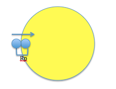
We begin by drawing out the situation described in the problem 

From the drawing we need to balance gravitational forces between the star and the planet both acting on the orbiting particle or satellite. It's important to note that the balance has to exist on all sides of the particle's orbit around the planet. \[\frac{G M_s}{(R_p - R)^2} - \frac{G M_s}{(R_p + R)^2} = \frac{G M_p}{R^2} \] Cancelling G and simplifying both sides we get \[\frac{4 M_s R_p R}{R_p^4 - 2 R_p^2 R^2 + R^4} = \frac{M_p}{R^2} \] Because R is much smaller than \(R_p\) we can simplify the left side of the equation to \[\frac{4 M_s R}{R^3} = \frac{M_p}{R^2} \] Then by rearranging to solve for R we get \[R = R_p (\frac{M_p}{4 M_s})^{\frac{1}{3}}\]However the true equation for Hill Sphere differs by a constant factor due to orbital rotation speeds and comes out to \[R = R_p (\frac{M_p}{3 M_s})^{\frac{1}{3}}\]

Plugging constants from the table into the equation above, we get \[R_{Earth} = 1.49*10^6 \space km \quad R_{Jupiter} = 5*10^7 \space km \quad R_{Neptune} = 1.15*10^8 \space km \]Comparing these values to the values for the furthest moon around each planet it becomes clear that each moon is well within the planet's Hill Sphere. 

Blog #23 - History of ISM

History of ISM

The interstellar medium, or ISM, is one of the more complicated phenomena in the universe. Interestingly, the first mention of ISM was back in 1626 quoted by English explorer Francis Bacon as he stated "The Interstellar Skie.. hath .. so much Affinity with the Starre, that there is a Rotation of that, as well as of the Starre." Later, English philosopher Robert Boyle (of Boyle's law) claimed "The inter-stellar part of heaven, which several of the modern Epicureans would have to be empty." 

These early reports showed that even with primitive technology, early philosophers and astronomers were able to deduce that the space between the stars and planets in the night sky was not mere emptiness. However, for centuries, scientists believed there was an luminiferous ether that moved light throughout the universe but did not have any quantitative data as to how electromagnetism or quantum physics operated. 

In 1904, after the advancement of absorption spectroscopy, Johannes Hartmann, a German physicist, made the first observation of cold diffuse matter. This matter, later to be described as the Interstellar Medium was found as Hartmann observed the light curves of Delta Orionis. He saw that the "k" line of calcium appeared far too faint given the observing conditions and surrounding spectra. He concluded that much of the light must have been absorbed before entering Earth's atmosphere. 

Within the next decade, research into the ISM exploded and various researchers helped categorize ISM as clouds with doppler shifts. Then the discovery of cosmic rays confirmed that with the incredibly number of stars in the Universe there could statistically not exist an absolute vacuum and some medium would need to exist to absorb and transfer the massive amounts of cosmic rays, ionized hydrogen, and other basic elements that exist throughout the universe.

Today NASA has developed much of the theory behind the ISM but still lacks the knowledge to fully develop the development, growth, and existence of ISM. We now know that ISM interacts with polycyclic aromatic hydrocarbons (PAHs) to create the earliest forms of organic matter that may help shape how the big bang developed into life as we know if today. If these connections are confirmed, ISM will truly be responsible for all life as we know it.

Blog #22 - Stromgren Sphere

Stromgren Sphere

A) Set up an equation of the size of a sphere that is ionized around a star assuming uniform photon flux in all directions, and uniform density in terms of the total ionization rate \( \eta\), the density \(n\) and the recombination cross section \(\alpha\). Assume that all recombinations result in photons that cannot ionize anything further. At steady state the total photoionization rate \(\eta\) is balance by the total recombination rate.

Given the steady state assumption, we can begin by solving for \(\eta\) the recombination rate, by simple unit conversion. We know from the previous post that the recombination rate, r, is \[r = n_e * n_p * \alpha \space [\frac{1}{s \cdot cm^3}] \]We know that the number of electrons and protons must be equal if the sphere is uniformly atomic hydrogen. \[n_e = n_p \rightarrow r = n^2 \alpha\]We want \(\eta\) in terms of \(\frac{1}{s}\) meaning we need to multiply by the volume of the total sphere, given that the ionization (and recombination) occurs equally in all directions. \[\eta = n^2 \alpha V = \frac{4}{3} \pi r_{ss}^3 n^2 \alpha \]Rearranging to solve for \(r_{ss}\), the radius of the Stromgren Sphere, we find \[r_{ss} = (\frac{3 \eta}{4 n^2 \alpha \pi})^{\frac{1}{3}}\]

B) Calculate the total number of ionizing photons emitted per second by the kind of star identified in the previous problem assuming its entire luminosity is due to photons with exactly the energy required for ionizing hydrogen atoms.

This problem asks us to solve \(\eta\) which is a rate in units \(\frac{photons}{second} \). To do this we relate the luminosity of the star from the previous problem to \(\eta\). We know that the luminosity is the amount of energy emitted by the surface of a star every second. \[L = 4 \pi r^2 \sigma T^4 \space [\frac{erg}{s}] \] From the given table we find that for an O type star (temperature >30,000K). \[r_{star} \approx 10*R_{\odot} = 6.96*10^{11} cm\]With this information we solve the luminosity \[L = 4 \pi r^2 \sigma T^4 \space [\frac{erg}{s}] = 3.92*10^{38} \frac{erg}{s}\]To convert this into the rate we need, we simply divide by the energy of a single ionizing photon, \(2.17*10^{-11} erg\). \[\eta = \frac{L}{2.17*10^{-11} erg} = 1.8*10^{49} \frac{photons}{second} \]

C) With information from (A) and (B), what is the size of a Stromgren Sphere around this kind of star assuming an initial hydrogen atom density of \(1 cm^{-3}\). The recombination rate \(\alpha = 3*10^{-9} cm^{-3} s^{-1}\). How does your answer compare to the HII region of Orion, which is ionized by a few massive stars and is 8pc across?

Plugging in the \(\eta\) from (B) into the equation for \(r_{ss}\) from (A) we can solve for the radius of the Stromgren Sphere. \[r_{ss} = (\frac{3 \eta}{4 n^2 \alpha \pi})^{\frac{1}{3}} = \frac{3 * 1.8 * 10^{49}}{4* 1^2 * 3*10^{-9} * \pi} = 1.57 * 10^{57} cm \approx 5pc \]Our answer is expectedly smaller than the Orion system which has a few massive stars ionizing the HII region.

D) Make a drawing of the Stromgren sphere surrounded by the neutral HI region. What is the size of the transition region at the edge of the Stromgren Sphere where atomic hydrogen and protons co-exist? How does the size of the transition region compare with the radius of the sphere? Does it make sense to think about the HI and HII regions as distinct?

From the drawing and the information given in the problem it becomes evident that to find the size of the transition area we must calculate the mean-free-path to find the width of the area in which hydrogen protons will be ionized by photons. If this path length is very large, the two areas could be considered distinct, whereas if it is small, much of the HI region will continue to be ionized by the photons that cross the transition region. We calculate mean-free-path \[l = \frac{1}{n * \alpha} \]Where n is the particle density and \(\alpha \) is the ionization cross-section as defined in the earlier section. \[l = \frac{1}{1*3*10^{-9}} \approx 3*10^8 cm\]This transition zone is significantly smaller than the the Stromgren radius of 5pc, thus we consider the two regions as non-distinct and expect interaction along the edge of the radius.

Blog #21 - Hydrogen Ionization

Hydrogen Ionization 

A) The most abundant species in the ISM outside of molecular clouds is atomic hydrogen. We need to determine how hydrogen is ionized in order to determine properties of the ISM. Make a drawing of the electronic energy levels of atomic hydrogen. Mark out the energy needed to excite an atom in its ground state to a free proton and electron. Illustrate what happens in the case of photoionization.

http://dev.physicslab.org/Document.aspx?doctype=3&filename=AtomicNuclear_BohrModelDerivation.xml

When the hydrogen atom receives enough energy from incoming light to jump up 13.6 eV in energy, it escapes it's atomic structure and ionizes into a proton and an electron. 

B) Remember that stars are blackbodies. Which kind of stars emit a majority of their protons with energies high enough to photoionize (excited the electron to freedom) ground state hydrogen. Give your answer in both stellar temperature, and letter classification. 

To solve for the temperature needed to create a 13.6 eV increase in energy we can simply use Planck's law and Wein's displacement law. First we know \[E = \frac{h c}{\lambda}\] which gives us \[13.6 eV = \frac{4.135*10^{-15} * 3*10^8}{\lambda} \rightarrow \lambda = 91.2 nm = 912 angstrom \]With this wavelength we can use the Wein displacement law to solve for temperature. \[\lambda T = 3 * 10^{-3} m \cdot K\] From here we can solve for temperature of our blackbody. \[T = \frac{3*10^{-3} m \cdot k}{91.2*10^{-9} m} = 32894 K \]This very high surface temperature gives the star an O Type classification on the Morgan-Keenan scale. 

C) The ionization cross section is \(10^{-17} cm^2 \). Calculate the photon flux assuming the you are sitting right next to the star from (B) and that the star is emitting all of its energy in the form of photons with the exact energy required to ionize atomic hydrogen. How does this time scale compare to the excited time scale of a hydrogen atom, \(10^{-9} s \)? Is it reasonable to assume that all hydrogen is at the ground state? 

We begin with the Stefan-Boltzmann law to relate the stellar flux to the temperature of the star. \[\sigma T^4 = F \rightarrow (5.67*10^{-5} \frac{erg}{s \cdot cm^2 \cdot K^4} * (32894 K)^4 = 6.64*10^{13} \frac{erg}{s \cdot cm^2} \] Using simple unit conversion we can find our timescale from this result by multiplying by an area (to cancel the cm^2) and dividing by an energy (to cancel the ergs).\[6.64*10^{13} \frac{erg}{s \cdot cm^2} * 10^{-17} cm^2 * \frac{1}{13.6eV = 2.18*10^{-11} erg} = 3.05*10^7 \frac{photons}{second} \]Converting this to a timescale through inversion we get \[3.05*10^7 \frac{photons}{second} = 3.28*10^{-8} \frac{seconds}{photon} \] This time scale is larger than the \(10^{-9}\) excited state lifetime meaning that the photon will almost always fall back to its ground state before the next photon has the chance to ionize the atom to its next energy level. 

D) Draw a recombination event. Set up an equation for the recombination rate, r (which has units of cm^3 s^-1), in terms of the number densities of photons, electrons (np and ne) and the rate coefficient \(\alpha\), which describes the efficiency at which a recombination occurs when an electron and proton collide. 

http://hendrix2.uoregon.edu/~imamura/123/lecture-6/recombination.jpg

To solve for the recombination rate, we simply need to match units. We know \[n_p = \frac{protons}{cm^3} \quad n_e = \frac{electrons}{cm^3} \quad \alpha = \frac{cm^3}{s}\] Thus if we want a rate in terms of \(\frac{1}{cm^3 \cdot s} \) we simply need to multiply the three terms. \[r = n_p * n_e * \alpha \]

Blog #20 - What is TRAPPIST?

What is TRAPPIST? 

A lot of excitement was generated on February 22, 2017 when NASA released a press statement announcing the founding of 7 exoplanets orbiting a star 12 parsecs from Earth. Using transit photometry, as discussed in earlier blog posts, the Transiting Planets and Planetesimals Small Telescope (TRAPPIST) was able to record the presence of 7 exoplanets around a single star, 5 of which appear to be in or around the habitable zone while 3 have roughly Earth-sized radii.

TRAPPIST is actually a system of two 60-cm reflective, optical telescopes. The first, TRAPPIST-South is located in the Chilean mountains at La Silla Observatory while TRAPPIST-North is located in the Atlas Mountains of Morocco. Despite their locations, both telescopes are controlled out of Liege, Belgium and operate under fully autonomous, robotic systems. The team of telescopes creates photometry data by observing when planets transit across their host stars, causing an observed drop in incoming flux. The plot below shows the process for determining the transit of a planet which helps determine its period, radius, and location around a star.

When it came to the 7 planets orbiting TRAPPIST-1, the photometry data was truling startling as the 7 planets all created well defined transit drops. Below is the aligned data for all 7 planets as well as the brightness plots and a schematic of the orbits for the star system. 

The bottom left image is the aligned 7 photometry plots with clear ingress and egress dips and corresponding transit depths. These images in conjunction with the TRAPPIST telescopes were imaged by the Spitzer Space Telescope. 

Blog #19 - Transiting Exoplanet pt. 2

Transiting Exoplanet pt. 2

2. Now draw the star projected on the sky, with a dark planet passing in front of the star along the star’s equator.

The picture above depicts a planet transiting in front of its host star as observed from Earth

(a) How does the depth of the transit depend on the physical properties of the star and planet? What is the depth of a Jupiter-sized planet transiting a Sun-like star?

The optical depth or, \(\delta F\), is solely dependent on the cross sectional areas of the planet and the star, thus the radius is the only physical property we care about when considering depth of transit. \[\delta F = \frac{A_p}{A_{\star}} = \frac{\pi R_p^2}{\pi R_{\star}^2} = \frac{R_p^2}{R_{\star}^2} \] From the previous problem we know for a Jupiter-sized planet and a Sun-sized star, \[R_{\star} \approx 10*R_p\]Substituting into the equation for optical depth, we get \[\delta F = \frac{R_p}{10 R_p} = 10 \% \space transit \space depth\]

(b) In terms of the physical properties of the planetary system, what is the transit duration, defined as the time for the planet’s center to pass from one limb of the star to the other?

We know that for an full transit to occur, the planet's center must travel a distance of \(2 R_{\star}\) if observing the planet as traveling along a line at the equator of the star. We can use the simple relation between distance, velocity, and time to get the total transit time. \[t = \frac{d}{v}\]and \[v = \frac{2 \pi a}{p} \]This gives us \[t = \frac{2 R_{\star} P}{2 \pi a}\]To get the answer in terms of solely physical properties we can convert the orbit period, P, to \[P = 2 \pi \sqrt{\frac{a^3}{MG}}\] leading to a final answer of \[t = 2 R_{\star} \sqrt{\frac{a}{M_{\star}G}} \]Where \(a\) is the semi-major axis, M is the mass of the star, and G is the universal gravity constant.

(c) What is the duration of “ingress” (from no transit to full transit) and “egress” (from full transit to no transit) in terms of the physical parameters of the planetary system?


We know that given a spherical star and planet, the time of ingress must equal the time of egress\[t_{ingress} = t_{egress} \]Following the same method as part (b) we can solve for the time for the planet to move across the star's surface the distance of one planetary radius equating to the ingress transit time as seen in the diagram below.

From this diagram we can solve the time of transit using the same relation of distance, velocity, and time. \[t = \frac{d}{v} = \frac{R_p}{\frac{2 \pi a}{P}} = R_p \sqrt{\frac{a}{M_{\star}G}}\]